Matt Mahoney, June 6, 2003, revised June 9, 2004
A multidimensional time series is modeled by approximating its path through state space with a sequence of boxes. A test point is anomalous if it is outside of any box, with a score depending on the distance from the nearest box. An algorithm for approximating N M-dimensional points using K M-dimensional boxes that runs in O(NM + N log N) time is described. Test time per point is O(KM) worst case, but can be approximated in O(M) time by maintaining the nearest box as a state variable. The method may be generalized to multiple training series by merging paths with no additional cost in testing time. Results are presented for Marotta valve solenoid current signatures.
In prior work, time series was modeled as a path through multidimensional space. A series of N points in M dimensions (including first and second derivatives) is approximated in O(NM + N log N) time as K linear segments through state space, scaled to a unit M-cube. A test point has an anomaly score equal to the square of the distance to the nearest point on the path. Path modeling was extended to multiple training series by finding the P nearest points in each of P paths to the test point and placing a bounding box around these P points. The anomaly score of the test point is the square of the distance from this bounding box.
Path modeling with bounding boxes runs in time O(PKM) time per test point with exhaustive testing of all segments in all paths, but can be approximated by testing only segments near the previously closest segment in each path, plus a few segments picked at random to break out of local minima. This approximation runs in O(PM) time.
Although box modeling has the same worst-case time complexity as path modeling (for both training and testing), testing is faster in the average case. Path modeling requires multiplication operations to compute the distance to the nearest line segment for every test point, whereas box modeling requires only comparison operations for the usual case where the test point is inside a box. Furthermore, once a box containing the test point is found, there is no need to test the remaining boxes. This means that exhaustive testing of all boxes in the path starting with the current box and iterating forward through the path will usually find a containing box on the first or second iteration. Thus, exhaustive testing has average case running time of O(M) rather than O(KM) (for P = 1 training path).
The goal of box approximation is to find a set of K M-dimensional boxes containing a path such that the total volume is minimized. If this goal is met, then the training path will have an anomaly score of 0, but the probability of a randomly chosen point having a nonzero score is maximized. Since this is a combinatorial problem, we choose a heuristic approach that is not optimal in either sense (the total volume is larger than the minimum possible, and some parts of the original path are outside of the boxes), but which gives good results in practice. The algorithm is as follows:
  Enclose each of the N - 1 pairs of adjacent training points in a box
  Repeat N - K - 1 times
    Remove the box with the lowest cost
    Extend the two neighboring boxes to include the center of the removed box
The cost of removing a box is the volume of the two expanded neighboring boxes minus the volume of the three original boxes. Note that the cost does not account for possible overlap with boxes elsewhere in the path. Also, the two boxes at the ends of the path are never removed. Thus, we require K >= 2.
Figure 1 illustrates the algorithm. The initial training series has N = 5 points in M = 2 dimensions. In each step, "d" indicates the next box to be deleted. For the step K = 4, the choice is arbitrary, as the two middle boxes have the same cost.
 x,y       y                y                y              y
 1,2     10|        /     10|      +-+     10|      +-+   10|     +--+
 3,4       |                |      | |       |      | |     |     |  |
 5,6      8|      /        8|    +-+-+      8|   +--+-+     |     |  |
 7,8       |                |    | |         |   | d|    6.5|+----+--+
 9,10     6|    /          6|  +-+-+         |   |  |       ||    |
           |                |  |d|          5|+--+--+       ||    |
          4|  /            4|+-+-+           ||  |          ||    |
           |                || |             ||  |          ||    |
          2|/              2|+-+            2|+--+         2|+----+
           |                |                |              |
           +----------x     +----------x     +----------x   +----------x
            1 3 5 7 9        1 3 5 7 9        1  4  7 9      1   5.5  9

     Input, N = 5              K = 4            K = 3          K = 2
                            volume = 12      volume = 22    volume = 32.5

                   Fig. 1.  Box approximation algorithm
Box approximation fails in the case where the path is flat over a region in one or more dimensions. In this case, all of the boxes will have a volume of 0, so the algorithm removes boxes arbitrarily. This problem can be overcome by adding a small positive number D to each dimension in the original set of boxes, for example, 0.001 of the range in each dimension. Since boxes may grow but are never shrunk in any dimension, it is impossible for any box to have a zero volume at any step in the algorithm.
Box approximation runs in O(MN + N log N) time by using a doubly linked heap (as in path approximation). The links point to neighboring boxes, and the heap is sorted by cost. When the lowest cost box at the front of the heap is removed, the neighbors are extended and their costs updated in O(M) time, and they are repositioned in the heap in O(log N) time.
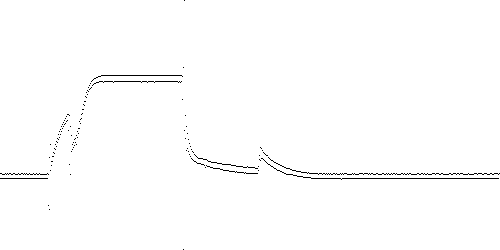
In practice, box approximation is applied to a time series after filtering and taking derivatives. Fig. 2 shows 1000 samples of solenoid current in a Marotta fuel control valve as it is cycled on and off during a 1 second period.

Fig. 2. TEK-0 solenoid current
Fig. 3 shows the same time series and its first two derivatives, where each of the three signals is filtered through a pair of digital low-pass RC filters with a time constant of T = 5 ms. Specifically, 3 signals are generated:
  y = F(F(x))           (black)
  dy = F(F(D(y)))       (red)
  ddy = F(F(D(dy)))     (green)
where F(x) denotes the filtering operation:
y[t] = ((T-1)y[t-1] + x[t]) / Twhere x[t] and y[t] are the input and output at time t, and T = 5. The derivative operation D(x) is:
y[t] = x[t] - x[t-1]
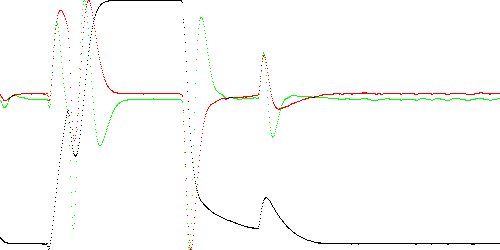
Fig. 3. Filtered TEK-0 solenoid current (black), first derivative (red), and second derivative (green)
Fig. 4 shows the path formed by these 3 time series. Current (y) increases upwards, the first derivative (dy) increases to the right, and the second derivative (ddy) increases toward the back of the cube. The red line corresponds to the rising edge of the waveform, and the green line to the falling edge. The two loops correspond to the spikes in the rising and falling edges. The flat sections of the time series correspond to the points at the bottom and top of the cube. For clarity, the "shadow" of the 3-D curve is traced on the bottom of the cube.
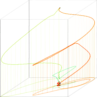
Fig. 4. TEK-0 path model
Fig. 5 shows box approximations of the path model using K = 1000, 100, and 20 boxes, and D = 0 (no adjustment to initial boxes). The change in color between K = 1000 and 100 is due to the removal of most of the tiny boxes at the top and bottom of the figure (the flat sections of Fig. 2). In all three paths, the colors transition smoothly through the spectrum from red to blue. The curved line connects the centers of the boxes.
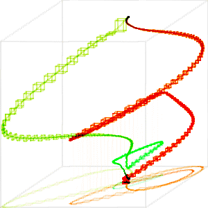
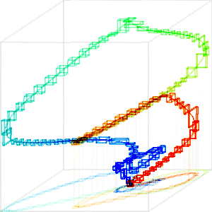
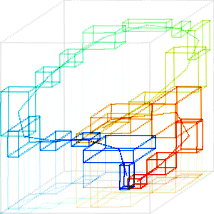
Fig. 5. Box approximation with K = 1000, 100, and 20 boxes with D = 0
The TEK 0 path lacks flat regions, so the box modeling algorithm works with no adjustment of the initial box dimensions (D = 0). Fig. 6 shows the effect of increasing D. Recall that D is the fraction of the range added to the radius (half width) to the initial set of N-1 boxes in each dimension.
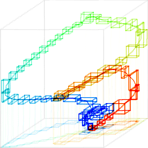
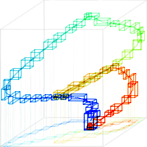
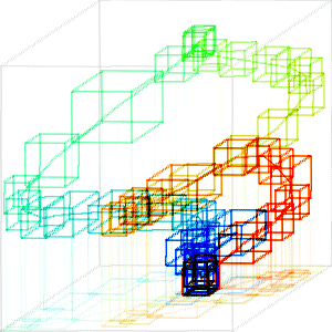
Fig. 6. Box approximation with K = 50 and D = 0.001, 0.01, and 0.05.
All of the above paths were sampled at the original rate of 1 ms (1000 samples). Because the data is low pass filtered, there is no need to sample faster than the Nyquist rate, roughly T = 5 ms (the time constants of the RC filter pairs) to accurately reconstruct the path. However, a low sampling rate can result in larger initial boxes because the data points along the path are more widely separated. Fig. 7 shows the effect of sampling at 5 ms, first with no approximation (K = 200, D = 0), then with approximation using K = 20, D = 0. Compare Fig. 7 with Fig. 5.
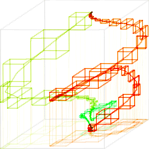
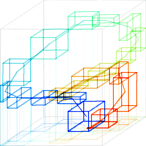
Fig. 7. Initial boxes (K = 200, D = 0) and approximation (K = 20, D = 0) with 5 ms sampling rate.
A test signal is anomalous if its path is not contained within the training boxes. If a test point is not within any box, then we assign an anomaly score of d2, where d is the Euclidean distance to the nearest box. For measurement purposes, we scale the training data (the centerrs of the original N-1 boxes) to a unit cube in M dimensions. Thus, the distance of any edge of the cube is 1, and the distance between diagonally opposite corners of this cube is M1/2.
If there is more than one path, then we use an approach similar to path modeling. We compute the anomaly score by placing a bounding box around the nearest training box in each path, then measure the distance to this bounding box. This means that a point between two paths will have an anomaly score of 0 because it will be contained in the bounding box. This allows for generalization to signals "between" the training data, but not outside.
                      path 1       path 2
                    +--+         +----+
                    |  |         |    |
                 +==+==+====+    |    |
                 I A|       +----+----+
              +--+--+       I    |
              |  I    t1    I    |
           +--+--+     +----+----+
           |  |  I     | B  I
        +--+--+  I     |    I
        |  |     +=====+====+
        +--+       |   |
                               t2

        Fig. 8.  Anomaly detection with multiple paths
If Fig. 8, the nearest box to test point t1 in path 1 is A. The nearest box in path 2 is B. If we enclose a bounding box around both A and B (thick lines), then t1 is inside this box, so its anomaly score is 0. The nearest boxes to test point t2 are also A and B, but in this case t2 is outside of the bounding box, so it receives an anomaly score equal to the square of the distance to the bounding box.
  Build a box model (as in Section 2)
  For each additional training point (pass 1)
    Label the point with the nearest box
  For each additional training point (pass 2)
    Expand the labeled box to enclose it
This algorithm guarantees that all of the additional training data would have an anomaly score of 0 if it were used as test data. Since the original training series might not have a 0 score, it is sometimes useful to include it again during merging.
One disadvantage of this algorithm is that the result depends on the training order. Ideally, the first series should be "average" behavior. Then we expand the model by supplying training data near the envelope of acceptable behavior. Fig. 9 and 10 illustrate the merge of TEK-0 and TEK-10. TEK-10 is abnormal in that it lacks spikes on the rising and falling edges (second waveform of Fig. 11 belo) indicating a stuck poppet. Consequently its path lacks loops on the rising and falling edges. Fig. 9 shows the box models for each path (K = 20 boxes, T = 5 ms filter time constant, S = 5 ms sampling rate). Fig. 10 shows the TEH-0 box model to fit TEK-10 on the left, and the TEK-10 model expanded to fit TEK-0 on the right.
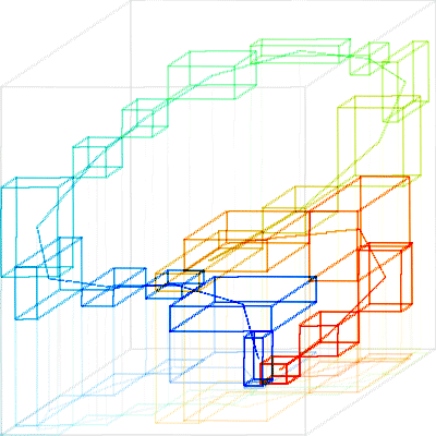
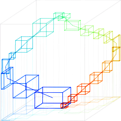
Fig. 9. Box models of TEK-0 (left) and TEK-10 (right)
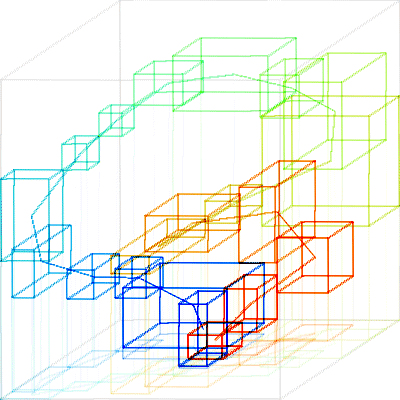
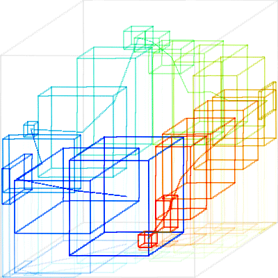
Fig. 10. Merged box models of TEK-0 and TEK-10 with TEK-0 as the base (left) and TEK-10 as the base (right)
Testing is as described as in Section 3 with a single path.
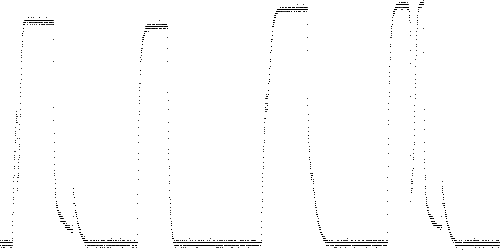
Fig. 11. Solenoid current for TEK 3, 10, 14, and 16.
The paths for these four series are shown in Fig. 12. TEK 3 (red) is normal. TEK 10 (yellow) deviates from normal on the rising and falling edges, which lacks the two loops corresponding to the spikes on these edges. TEK 14 (green) also deviates, in that the smaller spikes result in only small dimples in the path. TEK 16 (blue) has an extra loop from the top vertex corresponding to the dip in the middle of the "on" portion of the trace. It deviates from normal (red) on the rising edge but is normal on the falling edge.
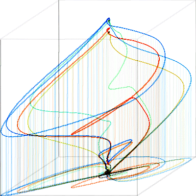
Fig. 12. Paths of TEK 3 (red), 10 (yellow), 14 (green), and 16 (blue).
The following results are obtained using the bounding box method of Section 3 after training on TEK 0 and TEK 1, with a filter time constant and sample rate of T = 5 ms (200 samples total), K = 30 or 50 boxes, and D = 0. The numbers shown are the total anomaly scores of all test points for each series. The tests pass because the normal scores for TEK 2-3 are lower in every case than the abnormal scores for TEK 10-17. The margin between the normal and abnormal traces improves as K is increased. Total run time (training and test) for each set is less than 1 second on a 750 MHz PC.
  TEK test, K = 30, D = 0, T = 5, M = 3

Training, TEK 0-1 (should be 0 scores)
0.121543
0.0884858
Test, normal, TEK 2-3 (should be low scores)
9.24486
11.8133
Test, abnormal, TEK 10-17 (should be high scores)
70.0613
41.1993
32.8128
164.049
246.016
187.402
428.623
146.779


  K = 50

Training, TEK 0-1 (should be 0 scores)
0.0294261
0.165668
Test, normal, TEK 2-3 (should be low scores)
26.0669
32.2325
Test, abnormal, TEK 10-17 (should be high scores)
298.19
191.929
136.712
536.437
919.156
684.437
991.166
496.824
The scores for TEK 0 and 1 are not 0 because the box approximation algorithm can move the training path slightly outside the boxes.
The test fails for K less than about 22 boxes. Results shown below are for K = 20. Note that TEK 12 has a lower score than TEK 2-3.
  K = 20

Training, TEK 0-1 (should be 0 scores)
0.067218
0.112195
Test, normal, TEK 2-3 (should be low scores)
4.4996
5.72594
Test, abnormal, TEK 10-17 (should be high scores)
10.6886
8.91267
3.40629
13.7626
30.7031
28.8332
117.316
31.7471
The filter time constant and sampling rate T = 5 sets the range of durations of the types of events we which to detect to approximately T to 10T. For the TEK data, we are interested in abnormal spikes on the rising and falling edges, which last about 10-100 ms. We are not interested in variations in the duration of the "on" phase, which is about 250 ms. At K = 50, the tests pass for T ranging from about 2 ms to 60 ms.
The following results were obtained using model merging as described in Section 4. TEK-0 was used as the base, which was then expanded using TEK-1 with parameter K = 20 boxes and all other parameters as in 5.1.1 (T = 5 ms, S = 5 ms sampling rate, M = 3).
Training, TEK 0-1 (should be 0 scores)
0.0476297
2.1294e-10
Test, normal, TEK 2-3 (should be low scores)
4.33956
5.5269  (TEK 3)
Test, abnormal, TEK 10-17 (should be high scores)
15.5264 (TEK 10)
11.0322
9.53502
28.7849
44.5081 (TEK 14)
40.7323
142.645 (TEK 16)
32.5858
In this case the test passes. For these parameters, the test passes with as few as K = 8 boxes. For K = 50, the range of T over which the test passes is still about 2 to 60 ms as in 5.1.1. Fig. 13 shows the anomaly scores of TEK 3, 10, 14, and 16 as a time series (smoothed with T = 10 for clarity).
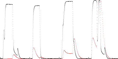
Fig. 13. Anomaly score (red) of TEK 3, 10, 14, and 16
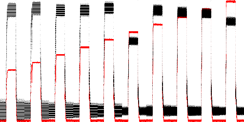
Fig. 14. VT1 shunt resistor current measurements (black) and Hall effect measurements (red) as voltage is increased from 14V to 32V under otherwise normal conditions.
Fig. 15 shows the effects of poppet blockage and high temperature at 32V. The poppet blockage causes the barely visible spikes in the rising and falling edges to decrease, as in the TEK data. High temperature causes the Hall effect current measurement, but not the shunt resistor measurement, to decrease.
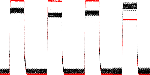
Fig. 15. Solenoid current at 32V under normal conditions, with poppet impedance of 4.5 and 9 mils, and hot (70 C).
Box modeling was evaluated by training on four series: 18V, 22V, 26V, and 30V at normal temperature with no poppet blockage. It was tested on all other series. There are two normal series not seen in training: 20V and 28V, which should receive low anomaly scores, and also 24V if only the Hall effect measurement is considered. Voltages outside this range (14V, 16V, 32V) should be detected as abnormal, as should all cases of poppet blockage or high temperature.
The box model was tested with a time constant and sampling rate of T = 50 samples (5 ms), K = 20 boxes, and D = 0. Because there are two signals, paths have 6 dimensions after taking derivatives. Results are shown below. The test passes because the highest score for a normal trace (0.18 for 30V) is less than the lowest score for an abnormal trace (0.84 for 32V hot). The latter case is hard to detect because high temperature has the same effect as low voltage (reducing Hall effect current) so the two anomalies almost cancel out.
  VT1 test, T = 50, K = 20, D = 0, M = 6

(18-30V, normal temperature and impedance)
Training data self anomaly scores (18, 22, 26, 30 V)
0.0805396
0.076466
0.0973737
0.187106
Test, new files under normal conditions (20, 28 V)
0.0378768
0.0865253
Test, abnormal in column 1, normal in column 2 (24 V)
3.9295
Test, low voltage (14, 16 V)
11.0939
1.71352
Test, high voltage (30V R0, R1, 45 mil, 90 mil, R2, T70)
4.20857
4.05036
8.00103
12.5518
3.90641
0.843828
Test, 4.5 mil impedance (16, 20, 24, 28 V)
3.08235
3.35808
6.69257
7.18148
Test, 9.0 mil impedance (16, 20, 24, 28 V)
2.75851
5.68192
6.70911
6.09589
Test, hot (T69-71, 16, 20, 24, 28 V)
26.9678
3.27082
0.906073
The test also passes when only Hall effect (input column 2) current is measured. In this case, the 24V series is considered normal. The highest normal score is 0.06 (30V). The lowest abnormal score is 0.14 (16V).
  VT1 test as above with M = 3

(18-30V, normal temperature and impedance)
Training data self anomaly scores (18, 22, 26, 30 V)
0.0278018
0.0280587
0.0201197
0.0643089
Test, new files under normal conditions (20, 28 V)
0.0280236
0.0247127
Test, abnormal in column 1, normal in column 2 (24 V)
0.0194749
Test, low voltage (14, 16 V)
0.911926
0.14259
Test, high voltage (30V R0, R1, 45 mil, 90 mil, R2, T70)
4.41524
4.25403
18.1224
13.1557
3.96361
0.312024
Test, 4.5 mil impedance (16, 20, 24, 28 V)
3.83658
2.79344
13.1505
12.1946
Test, 9.0 mil impedance (16, 20, 24, 28 V)
0.581352
3.32735
4.68045
4.2556
Test, hot (T69-71, 16, 20, 24, 28 V)
3.10201
0.288447
0.226096
0.283422
Total run time for each of the two tests is 8.5 seconds using both signals and 7 seconds using only Hall effect current.
  VT1 test, T = 50, K = 20, D = 0, M = 6

Training data self anomaly scores (18, 22, 26, 30 V)
1.19157e-10
2.6098e-10
3.10411e-12
3.00228e-10
Test, new files under normal conditions (20, 28 V)
0.0902655
0.253344
Test, abnormal in column 1, normal in column 2 (24 V)
12.1123
Test, low voltage (14, 16 V)
36.3152
4.97423
Test, high voltage (30V R0, R1, 45 mil, 90 mil, R2, T70)
9.4239
5.22137
18.9952
53.8517
4.63917
2.26905
Test, 4.5 mil impedance (16, 20, 24, 28 V)
35.0365
15.1541
11.3805
35.494
Test, 9.0 mil impedance (16, 20, 24, 28 V)
8.10408
39.2326
35.6864
33.1316
Test, hot (T69-71, 16, 20, 24, 28 V)
46.8402
7.83607
1.3921
1.70719
Box modeling is faster than path modeling, although in the actual implementations used in these experiments, the difference is small. Test time is O(MK) worst case and O(M) average case, compared to O(PMK) for path modeling with exhaustive testing. (for P paths, M, dimensions, and K boxes per path) Evauation usually stops when the current or next box in the path encloses the test point. Both box and path modeling are able to generalize across training sets and detect subtle anomalies in the VT1 data.
Box modeling has not been tested on complex, high frequency signals, in which the path contains many loops that are not easily modeled as a sequence of boxes. Future work will be to optimize models by removing or merging redundant, overlapping boxes.