Matt Mahoney
Oct. 10, 2003
In prior work, it was shown that data compression of solenoid current traces detects one set of forced failures in a valve used in the space shuttle program. A detection occurs when the incremental compression of the test trace after training on (compressing) a normal trace is poorer than the incremental compression of a second normal trace. This technique assigns an anomaly score to the entire trace of (C(xy)-C(x))/C(y) to test trace y relative to training (normal) trace x, where C(.) denotes compressed file size.
The training trace was one of two normal traces, TEK-0 or TEK-1, and the test traces were forced failures: TEK-2, 3, 5, 10, 11, 15, 16, or 17. For GZIP and PAQ3, all of the test traces have higher anomaly scores than TEK-0 or 1 when trained on the other normal trace (TEK-1 or 0). For RK using maximum compresion and delta coding (-mx3 -fd1), only TEK-15 has a lower anomaly score than the normal test trace. The traces are discretized so that each of the 1000 1ms current samples in each trace are represented by one byte.
This method has the drawback that anomalous points within the trace cannot be identified, because a score is assigned only to the entire trace. To rectify this, PAQ3 was modified to output a trace of instataneous compression. For each input byte, it outputs a value representing the number of output bytes averaged over an exponentially decaying window with a time constant of 16 input bytes. Regions of poor compression after training, relative to compression without training, should indicate anomalous points. PAQ3 was chosen because source code is available.
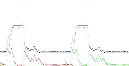
The graphs on this page plot instantaneous compression over time for 10 pairs of concatenated traces with training (red) and without training (green). The left side is always TEK-0, which is normal, and serves to train the compressor. The right side is one of the 10 traces. The X axis represents time, at 4 samples (4 ms) per pixel (range 2000 samples, or 500 pixels). The black line represents the measured value in the range -1 to 4 A on the Y axis.
The instantaneous compression is on a scale of 0% (bottom) to 400% (top, e.g. expansion to 4 output bytes per input byte). Compression is obtained when the area under the red or green line is less than 1/4 of the total area of the graph.
The red line shows instantaneous compression on the two traces shown by the black line. The green line shows instantaneous compression when the first (training) trace is replaced with 1000 zero bytes (essentially no training). The instantaneous anomaly score is the height of the red line divided by the height of the green line. Normally the green line should be higher. An anomalous region is indicated by the red line close to or above the green line.

TEK 0 - 0. The training and test data are identical. Because the test data is an exact copy of the training data, it is entirely redundant to the compressor, so compression is nearly perfect, indicated by the smooth red line at the bottom. The green line shows no training effect, e.g. it has the same shape as the red line on the left. The region between the red and green lines on the right side is very large, indicating an anomaly score of close to 0 (score = area under red / area under green).
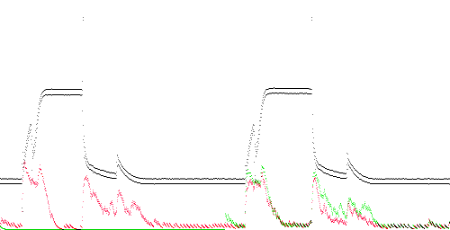
TEK 0 - 1. The training data is TEK-0 and the test data is TEK-1. Both traces are normal, but not identical. Compression is somewhat improved on the second trace because the compressor is able to use the statistics of the first trace as a model. Compression is poorest where either trace rises or falls rapidly. However these areas show a gap between the red and green lines, indicating that training improved compression in these regions (e.g. normal behavior).
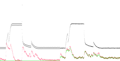
TEK 0 - 2. The training data is TEK-0 (normal) and the test data is TEK-2. The test trace is abnormal in that it lacks a sharp spike and overshoot at the falling edge. However, compression does not detect this. Instead it detects the absence of a 500 Hz noise component which is present throughout the training trace (alternating +0.04 and -0.04 values). This is indicated by a high anomaly score (red = green) throughout the trace.
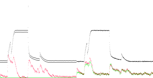
TEK 0 - 3. Similar to TEK 2.
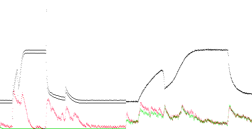
TEK 0 - 5. The slowly rising edge is clearly anomalous, and this region compresses poorly. More importantly, training hurts compression especially on the first rising edge, where the anomaly score is greater than 1 (red line above the green).
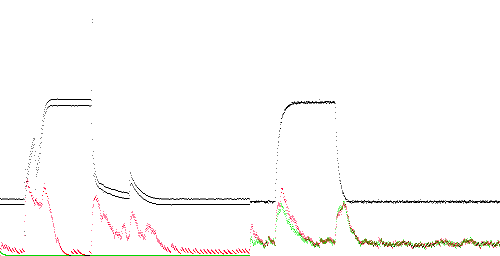
TEK 0 - 10. Poor compression appears due to the absence of 500 Hz noise, as in most of the traces below. However, the anomaly score is highest on the rising edge, which lacks the spike found in the training data.
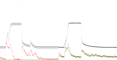
TEK 0 - 11. The anomaly score is highest at the start of the rising edge, which does not rise quickly enough.
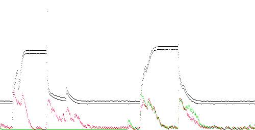
TEK 0 - 15. The 500 Hz noise in the training trace also appears in the test trace. This trace received the lowest anomaly score of all the abnormal traces, although still higher than TEK 1. The anomaly score is highest around the top of the rising edge and lowest around the bottom of the falling edge.
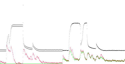
TEK 0 - 16. There are several places where the anomaly score is greater than 1 (red above green).
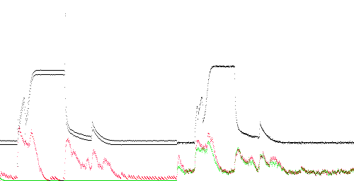
TEK 0 - 17. Again, there are high anomaly scores, especially on the rising edge.
PAQ3 is able to identify anomalous regions of the test traces. In most cases, peaks in instantaneous poor compression occur around rising and falling edges regardless of the location of anomalies, but differences between trained and untrained compression occur only when these edges are anomalous. Often, the score is higher than 1 (training hurts compression). This is not seen in the normal test trace.
Some of the anomaly detection may be due to the absence of 500 Hz noise in most of the abnormal samples (other than TEK-15). This is probably a test artifact and not an important feature of the forced failure.
PAQ3 is designed to compress text, not analog data. In particular, it treats byte values as nominal rather than continuous attributes, and does not generalize to adjacent values. Another problem is that it, like most programs, trains continuously, even on the test data. This suggests that the modeling could be improved. Recommendations are as follows:
Because the traces have low entropy (a few hundred bytes at most), their models should be expressable in SCL.