Matt Mahoney, Mar. 28, 2003
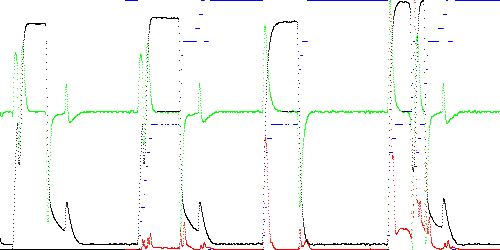
In Fig. 1 below, 4 time series (TEK00000, TEK00003, TEK00012, and TEK00016) are modeled and tested. The first waveform is a normal 1000 sample trace of solenoid current in a Marotta fuel control valve used in the Space Shuttle program as the valve is energized and de-energized over a 1 second period. The next three are test waveforms, which are compared to TEK00000. TEK00003 is almost normal. TEK00012 is the result of a jammed poppet, lacking spikes on the rising and falling edges normally caused by solenoid movement. In TEK00012 poppet movement is delayed but the falling edge is normal. The data was tested using TSAD4 with parameters T = 5 ms filter delay, M = 3 dimensions, and K = 20 path vertices.
In Fig. 1, the black line is the time series, green is the first derivative, red is the instantaneous anomaly score, and the blue stairstep is the number of closest training path segment to the test point. Maximum and total anomaly scores are listed below. Note that the almost normal TEK00003 has the lowest scores.
Anomaly Scores                      Maximum      Total
TEK00003.CSV                        0.012488     0.938373
TEK00012.CSV                        0.051081     1.981646
TEK00016.CSV                        0.113192     8.086108

Fig. 1. Anomaly scores (red) for TEK00000 (training), TEK00003 (near normal), TEK00012 (jammed poppet), and TEK00016 (delayed poppet movement). The data is black and the first derivative is green. The nearest training path segment is shown in blue.
Fig. 2 below shows the training (black) and 3 test paths (red, green, and blue) in 3 dimensions without piecewise approximation. The path shows x upward, dx to the right, and ddx toward the back. Each path starts at the bottom center and move counterclockwise, spending most of its time at the bottom and top centers (representing the flat sections of the time series). The two smaller loops represent the spikes on the rising and falling edges.
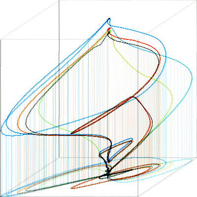
Fig. 2. Model path (TEK00000, black) and test paths (red = TEK0003, green = TEK00012, blue = TEK0016). Dimensions: x = up, dx = right, ddx = back.
Note that TEK00003 (red) closely follows the model (black). TEK00012 (green) lacks the two smaller loops corresponding to the spikes on the rising and falling edges. TEK00016 (blue) lacks a rising edge loop, and has an extra loop from the top point corresponding to the dip in the middle of the waveform.
Fig. 3 shows the approximation of the training path with K = 20 vertices in black. The actual path is shown in color, moving from red (rising edge) to green (falling edge).
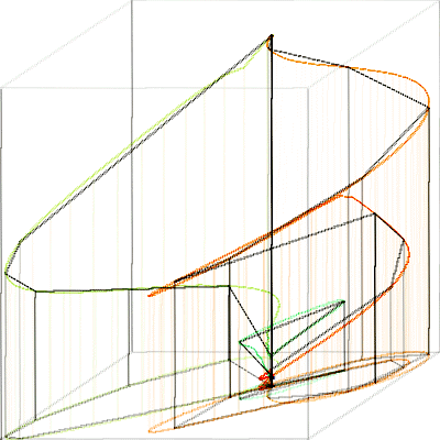
Fig. 3a. TEK00000 model path (color) and approximation (black) with K = 20 vertices. (Figure produced with xygraph.cpp).
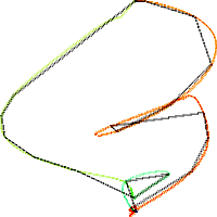
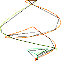
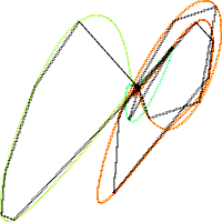
3b. Front view (dx by x). 3c. Right side view (ddx by x). 3d. Top view (dx by ddx).
TSAD4 by default models a test point by comparing it to every path segment, which takes O(MK) time. However, as can be seen in Fig. 1, the closest segment tends to advance sequentially, although in the case of the middle dip in TEK00016 it moves backwards for awhile. This suggests a faster O(M) test strategy of only testing the segments near the currently closest segment. However this can cause the state to become "stuck" in a local minimum. In Fig. 4 below, only the current and next segment are tested. If the next segment is closer, then the state is advanced. As can be seen, TEK00012 becomes stuck in states 3 and 5, and TEK00016 gets stuck in state 3 until after the center dip. This results in abnormally high anomaly scores. Note the high false anomaly score after the trailing edge TEK00012.
Anomaly score                       Maximum         Total
TEK00003.CSV                        0.012488     1.080274
TEK00012.CSV                        0.347073   175.150220
TEK00016.CSV                        0.460096    79.387458
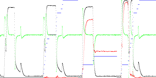
Fig. 4. Anomaly score (red) and state (blue) when only the current and next segment is examined (TSAD4 parameter R = 0).
If we relax the constraints by checking the nearest 4 segments (previous, current, and next two) then the state is better able to track the nearest segment at the cost of doubling test time.
Anomaly score                       Maximum         Total
TEK00003.CSV                        0.012488     1.080097
TEK00012.CSV                        0.281292    12.457304
TEK00016.CSV                        0.912214    92.647794
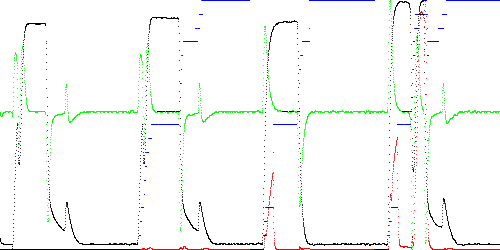
Fig. 5. Anomaly score (red) and state (blue) when examining the 4 nearest segments (TSAD4 parameter R = 1).
However this strategy fails when the approximation is improved. When K = 50 seggments, the state again becomes stuck. Compare Fig. 6 below with Fig. 4.
Anomaly score                       Maximum         Total
TEK00003.CSV                        0.008190     0.331296
TEK00012.CSV                        0.269940   156.064942
TEK00016.CSV                        0.373817    63.146571
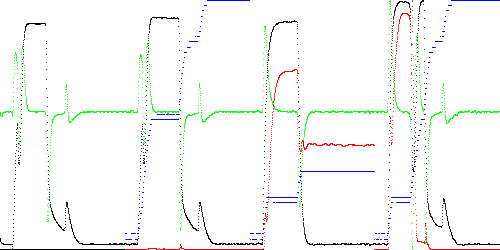
Fig. 6. Anomaly score (red) and state (blue) when examining the 4 nearest segments with K = 50 vertices.
The problem is solved by checking one segment picked at random in addition to the current and next segment. The next state becomes whichever of the three segments is closest. Results are below.
Anomaly score                       Maximum         Total
TEK00003.CSV                        0.008190     0.398291
TEK00012.CSV                        0.083796     2.719370
TEK00016.CSV                        0.198216    10.415991
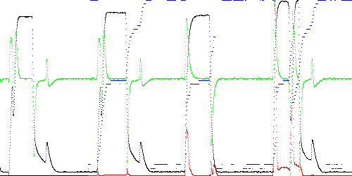
Fig. 7. Anomaly score (red) and state (blue) when examining the current, next, and a random segments with K = 50 vertices (TSAD parameter R = 2).
TSAD4 was trained on battery charger simulation (high sample rate) run21 to run30 and tested on run31 to run40. TSAD4 parameters are:
  N = 10479 samples (run21 to run30)
  C = 3 (battery 1 voltage)
  T = 5 sample filter time constant
  K = 1000 vertex training path approximation
  M = 3 dimensions
  R = 4 (exhaustive distance test to all segments in path)
  S = 1 (no subsampling)
Training time is 0.4 sec. and test time is 2.9 sec. for 10478 test points on a 750 MHz PC. Results are below. All traces except run32 appear to be abnormal.
Anomaly score                         Maximum         Total
run31_high1_noise0.txt                0.314834   244.453919
run32_high2_noise0.txt                1.545234    25.543668
run33_high12_noise0.txt               0.314516   210.654780
run34_low1_noise0.txt                 3.348493    53.009543
run35_low2_noise0.txt                 0.002243     1.650604
run36_high1_noise500.txt              0.219307     6.895755
run37_high2_noise500.txt              0.030710     3.458291
run38_high12_noise500.txt             0.007737     3.111194
run39_low1_noise500.txt               0.009452     3.073528
run40_low2_noise500.txt               0.182005     5.040834
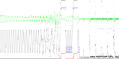
Fig. 8. Battery charger simulation. Black = battery 1 voltage, green = derivative, red = anomaly score, blue = state.
Training and test path are shown below. The large red and yellow loops are run31 and run33.
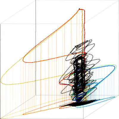
Fig. 9. Training path (black) and test path (transitions from red = run31 to blue = run40).
The large number of approximation vertices are needed because of the complexity of the training data. Below is the training path approximated to K = 500 vertices. The path moves from red to blue.
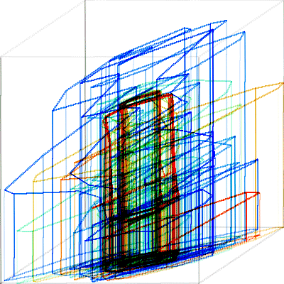
Fig. 10. Training path approximation (K = 500) for run21 (red) through run30 (blue).
In prior work, a path is approximated by successively removing vertices with the lowest cost, where the cost of removing point B in the vertex sequence ABC is dh2, where d is the distance from A to C, and h is the distance from B to the closest point on AC. (Fig. 10). This cost would be proportional to the (false) anomaly score of d points distributed along ABC.
                            B                   B
                           /|\                 / \
                          / | \               /   \
                         /  |  \          A'-a--+--c--C'
                        /   |h  \           /   t   \
                       /  d |    \         /         \
                      A ----+---- C       A           C
                            t
Fig. 10a. Cost of removing point B is dh2. 10b. Best fit to ABC is by A'C'.
In Fig. 10a, the total cost of d test points evenly distributed along the path ABC is proportional to the integral from A to C of dh2 = dh2/3 if we approximate the path by AC. However we can reduce the cost to dh2/6 if we approximate the path by the line segment A'C' formed by shifting AC 1/2 the distance to B along the line tB, where t is the closest point on AC to B. This can easily be seen to be optimal by the symmetry of the triangles AA'a and atB, and also by the triangles CC'c and ctB.
Unfortunately adjusting the vertices A' and C' introduces an error along the two paths to neighboring vertices. To solve this problem, we instead shift AC by 1/4 the distance to B, rather than 1/2. This has approximately the same net effect because a vertex is then moved twice when each of its neighbors are removed, for a total of 1/2 the average distance in the direction of the two removed neighbors (Fig. 11).
                                    C'
                             B     / \     D
                              +---/-+-\---+
                              |  /  C  \  |
                              | /t1   t2\ |
                              |/         \|
                              /           \
                             /|           |\
                            / |           | \
                           A' A           E  E'
Fig. 11. Approximation of ABCDE by A'C'E' using path fitting. Vertex C is moved twice by the removal of vertices B and D; 1/4 the distance from t1 to B and 1/4 the distance from t2 to D.
Fig. 12 shows TEK00000 approximated with K = 20 vertices (black), first without adjusting the remaining vertices, and then with adjustment as described.
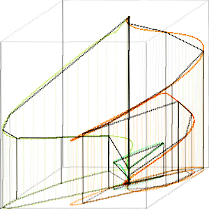
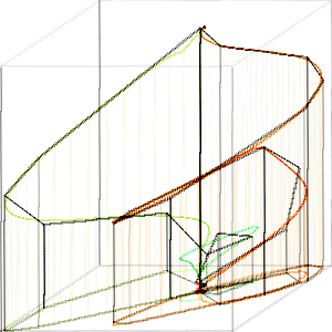
Fig. 12. TEK00000 path (red to green) approximated with K = 20 vertices by vertex removal (left). Approximation with path fitting (right).
The table below gives the anomaly score for TEK00000 when trained on itself as K is varied using vertex removal and path fitting. For large K, path fitting gives a better approximation as indicated by a lower anomaly score (which ideally should be 0). However, for small K, vertex removal gives a better approximation. The parameters are T = 5 samples, M = 3 dimensions, with exhaustive testing to all modeled segments.
Table. Maximum and total self-anomaly scores for TEK00000 (T=5, M=3) as K is varied from 200 to 20 segments using vertex removal or path fitting.
      Vertex removal             Path fitting
K     Maximum      Total         Maximum      Total
200   0.000008     0.000656      0.000005     0.000350
100   0.000057     0.005802      0.000019     0.003903
50    0.000345     0.027968      0.000542     0.025327
20    0.010298     0.601229      0.015872     0.961845
Fig. 13 below shows the self anomaly score for both cases when K = 50.
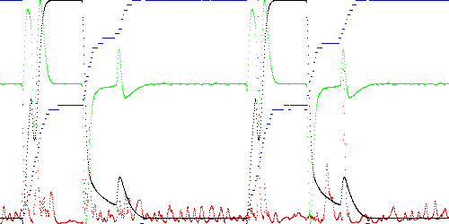
Fig. 13. Self anomaly score for TEK00000 (T=5, M=3, K=50, exhaustive testing) using path approximation by vertex removal (left) and path fitting (right). Key: black = x, green = dx, blue = state (closest segment), red = anomaly score.
On the TEK data, both models detect all anomalies by maximum and total score at K = 20 using fast testing. Parameters are T=5, M=3, R=3 or 11 (test previous, current, next 2 segments and one random segment). The model is trained on TEK00000. We consider TEK00001, TEK00002, and TEK00003 to be normal and all others abnormal, with TEK00001 the "most normal". The three normal traces have the lowest scores maximum and total scores. TEK00000 has the lowest total score of all (but not the lowest maximum score when using vertex removal). Test time is 0.02 seconds per trace on a 750 MHz PC (20 uS per test point).
Table. TEK anomaly scores using vertex removal and path fitting.
Anomaly scores, vertex removal      Maximum      Total
TEK00001.CSV                        0.013979     0.791604
TEK00002.CSV                        0.014103     1.097410
TEK00003.CSV                        0.012488     1.011889
TEK00010.CSV                        0.102027     2.981722
TEK00011.CSV                        0.067024     2.284380
TEK00012.CSV                        0.056211     2.100539
TEK00013.CSV                        0.057947     3.658688
TEK00014.CSV                        0.094561     6.007358
TEK00015.CSV                        0.072321     5.429257
TEK00016.CSV                        0.194060     9.394035
TEK00017.CSV                        0.042144     2.990856

Anomaly scores, path fitting        Maximum      Total
TEK00001.CSV                        0.014257     1.023932
TEK00002.CSV                        0.015712     1.275224
TEK00003.CSV                        0.015895     1.269365
TEK00010.CSV                        0.089830     2.824168
TEK00011.CSV                        0.062479     2.078511
TEK00012.CSV                        0.076915     3.009204
TEK00013.CSV                        0.040030     3.411337
TEK00014.CSV                        0.062185     5.293907
TEK00015.CSV                        0.046245     4.871815
TEK00016.CSV                        0.174138     8.052402
TEK00017.CSV                        0.053468     3.291609
The table below compares both modeling methods on VT1. Parameters are N = 40000 training points (V37898 V32 T21 R00s.txt and V37898 V32 T21 R01s.txt), C = 2 (Hall effect sensor), T = 50 sample filter time constant (5 ms), K = 50 segments, M = 3 dimensions (x, dx, ddx), R = 3 or 11 (fast testing using vertex removal or path fitting), S = 1 (no subsampling). In both cases, the normal trace, V37898 V32 T22 R02s.txt, has the lowest maximum and total anomaly score. Testing time is 23 uS per test point.
Anomaly scores, vertex removal     Maximum      Total
V37898 V32 T22 R02s.txt            0.001919     0.640254 (normal)
V37898 V32 T70 R03s.txt            0.054822   272.373455 (hot)
V37898 V32 T22 imp045 R01s.txt     0.006193     2.396629 (impeded)
V37898 V32 T22 imp09 R01s.txt      0.013796     5.527465 (impeded)
V37898 V30 T21 R00s.txt            0.004696    16.018069 (30 V)

Anomaly scores, path fitting       Maximum      Total
V37898 V32 T22 R02s.txt            0.001133     1.517164
V37898 V32 T70 R03s.txt            0.053374   269.048569
V37898 V32 T22 imp045 R01s.txt     0.006872     3.963795
V37898 V32 T22 imp09 R01s.txt      0.014203     7.076554
V37898 V30 T21 R00s.txt            0.004965    14.347913
Path model testing in M dimensions with state requires O(M) time per test point, as opposed to O(KM) for exhaustively testing all K path segments. Recovery from local minima requires O(K) time on average, but there is still a tradeoff. As the model accuracy (K) increases, run time now remains constant but recovery time from transient anomalies increases.