Matt Mahoney
Mar. 19, 2004
In prior work, a time series of n points was modeled by storing the path formed in m-dimensional space by the data and its first m - 1 derivatives. Each coordinate is low-pass filtered with a time constant T to remove noise and to allow comparison of the training and test data over a "fuzzy sliding window" with a size on the order of T. The configuration of the anomaly detector for m = 3 dimensions is shown in Figure 1.
                    x                   dx                  ddx
input -> LP -> LP --+--> D -> LP -> LP --+--> D -> LP -> LP -+
                    |                    |                   |
                    V                    V                   V
                +-----------------------------------------------+
                |               Anomaly Detector                |-> LP --> score
                +-----------------------------------------------+

          Fig. 1.  Path model anomaly detector in m = 3 dimensions.
In Fig. 1, x, dx, and ddx are the filtered input data and its first two derivatives, respectively. The low pass filtered data LP(t) as a function of input xt at time t is given by:
LP(t) = ((T-1)LP(t-1) + xt) / TDifferentiation of input xt is given by:
D(t) = xt - xt-1
A time series is modeled by storing the path traced by the n training points in m dimensions (x, dx, ddx for m = 3) in m-dimensional space, scaling the path to fit a unit m-cube. A test point is assigned an anomaly score equal to the square of the Euclidean distance to the nearest point on the path. Previously, this was estimated by comparing a test point to each of the n training points and taking the minimum distance. If a test trace has n points, then testing time is O(n2).
We can speed up testing by using a piecewise linear approximation of the training data. We approximate the path using k-1 line segments defined by k vertices. A point is tested by finding the closest line segment, which takes O(nk) time, where k << n.
Although we have previously developed a time series segmenter, GECKO [1], it is unsuitable for this purpose because GECKO finds second order polynomial segments (parabolas) rather than straight lines. Rather, we take the approach of greedily removing n-k vertices from the original path of n vertices, such that we always remove the vertex that introduces the smallest approximation error. For 3 consecutive points A-B-C, the error for point B is defined as:
  error(B) = |AC|d2                                     (1)
    where |AC| = length of line segment AC
    and d = distance from B to the closest point on AC
We justify this definition because a series of points
evenly spaced along A-B-C would
have an anomaly score approximately proportional to error(B), at least
when ABC is nearly a straight line.
                  B
                 / \
                A   C           A---B---C       A-------C
               /     \         /         \     /         \

             error(B) large   error(B) small   After removal

  Fig. 2.  Path ABC.  In the second drawing, B has a lower error and
  is therefore a better candidate for removal.
The algorithm for piecewise linear approximation of n points x0
though xn-1 to an approximation using k vertices is as follows:
  Repeat n - k times
    find xi such that 0 < i < n-1 and error(xi) is minimum
    remove xi
Note that the endpoints x0 and xn-1 are never removed.
A naive implementation would require O(n2) run time. However an O(n log n) algorithm is possible by storing the vertices in a doubly linked heap. Each vertex xi has a pointer to its neighbors, xi-1 and xi+1 in a doubly linked list. Each of the n-2 vertices that is a candidate for removal (all but the two endpoints) also has an associated error(xi) and is placed on a heap, a binary tree such that each vertex has a smaller error than either of its children. Thus, the next vertex to be removed is at the root of the heap. After a vertex is removed, we recompute the error for its neighbors and move them up or down the tree to restore the heap propery.
A heap can be efficiently represented without pointers by using an array A, such that the root is A[1] and the children of node A[i] are located at A[2i] and A[2i+1]. It is convenient to place the two endpoints in A[0] and A[n-1] outside the heap, which has an initial size of n-2. The doubly linked list is initialized so that A[i] points to A[i-1] and A[i+1]. When elements are moved to maintain the heap property, we adjust the pointers of elements that point to them. The algorithm is now as follows:
  store x0...xn-1 in a doubly linked list in A[0..n-1]
  for i = (n-2)/2 downto 1    (make A[1..n-2] a heap of size n-2 rooted at A[1])
    fix(i)
  for i = 1 to n-2
    compute error(xi)
  repeat until heap size = k - 2
    remove vertex xi from root of heap and from linked list
    recompute error(xi-1)
    fix(xi-1)
    recompute error(xi+1)
    fix(xi+1)
  output k elements of linked list
fix(i) means to restore the heap properties at node i, such that the
error is greater than its parent and smaller than its children. This
is a standard heap operation except that when an element is moved the
two linked list pointers to it must be updated. This requires O(log n)
time.
  fix(i)
    if error(i) < error(parent(i))
      swap(i, parent(i))
      fix(parent(i))
    else if error(i) > error(left(i)) or error(right(i))
      smallest = child with smaller error
      swap(i, smallest)
      fix(smallest)
Removing the root node is also O(log n):
  remove root from linked list
  swap(root, last element of heap array)
  heapsize = heapsize - 1
  fix(root)
Test time is O(nk) and is independent of the algorithm used to perform the piecewise approximation. A smaller value of k will result in faster testing, but a less accurate model. We justify the need for the user to select the parameter k on the grounds that test speed might be critical (as opposed to training speed) and therefore should be controllable by the user.
The algorithm has been implemented as tsad4.cpp.
TSAD4 was tested on the following data:
The TEK files TEK00000-TEK00003 and TEK00010-TEK00017 were tested using the following TSAD4 parameters
  n = 1000 training samples (TEK00000 only)
  C = 2 (column 2, current)
  T = 5 (low pass filter time constant = 5 samples = 5 ms)
  k = 20 line segment approximation
  m = 3 dimensions
  S = 1 sample rate (no samples skipped)
Table 1 shows the path model constructed by TSAD4. Each row is one vertex in the path. The time to construct the path model on a 750 MHz Duron (WinMe, g++ -O 2.95.2) was too fast to measure (less than 0.06 seconds).
Table 1.  TSAD4 path model for k = 20 (column headers added for clarity).

   t        xt             dxt             ddxt
  ---   ---------       ---------       ---------
    0   -0.008800       -0.000352       -0.000014
  114   0.642340        0.051950        0.003650
  123   1.278304        0.067386        0.002636
  131   1.750256        0.063092        0.000580
  147   1.493086        -0.022823       -0.005822
  158   1.396347        -0.017624       -0.001475
  166   1.896726        0.032341        0.003738
  175   2.651816        0.070459        0.004516
  191   3.553497        0.055307        -0.000756
  214   3.842302        0.009423        -0.001662
  259   3.861490        0.000045        -0.000020
  379   2.073069        -0.113553       -0.007284
  382   1.683617        -0.125006       -0.007022
  386   1.287922        -0.121739       -0.004702
  392   0.910673        -0.094554       0.000076
  400   0.648827        -0.054320       0.003693
  511   0.142311        -0.001392       0.000076
  529   0.593674        0.031034        0.002280
  550   0.455920        -0.008946       -0.001753
  999   -0.105000       0.000312        0.000034
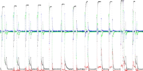
The output of TSAD4 is a column of m + 1 numbers: x, anomaly score, and the derivatives (dx and ddx for m = 3). This data is shown graphed (using the lgraph program) in Figure 3. The first waveform is the training data, TEK00000, which has an anomaly score of 0. Execution time to test 11,000 points was 0.27 seconds.

Fig. 3. Anomaly score (red) for training and test data (black = x, green = dx, blue = ddx). The 12 waveforms are TEK00000 (training), TEK00001 (normal), and 10 abnormal traces.
Table 2 below shown the peak and total anomaly score for each test trace. Note that the both scores are lower for the normal trace than for any abnormal trace.
Table 2.  TEK peak and total anomaly scores for k = 20, training on TEK00000.

k = 20                              Maximum      Total anomaly score
---------------                     --------     -------------------
TEK00001.CSV                        0.009874     0.641225 (normal)
TEK00002.CSV                        0.011808     0.907443
TEK00003.CSV                        0.012488     0.938224
TEK00010.CSV                        0.086664     2.610743
TEK00011.CSV                        0.022413     1.633306
TEK00012.CSV                        0.051081     1.982489
TEK00013.CSV                        0.039696     2.999528
TEK00014.CSV                        0.058897     5.265273
TEK00015.CSV                        0.058788     4.954365
TEK00016.CSV                        0.113192     8.085994
TEK00017.CSV                        0.040644     2.834691
Since testing time is O(nk), there is a tradeoff between run time and modeling accuracy in the selection of k. For this data, anomaly detection degrades unacceptably for k less than about 15-20. Table 3 shows the maximum and total anomaly scores for k = 1000, 50, and 15. For k = 15, the normal trace anomaly scores are almost as high as the abnormal traces.
Table 3.  TEK maximum and total anomaly scores for k = 1000, 50, and 15.

k = 1000 (no approximation)         Maximum      Total anomaly score
---------------                     --------     -------------------
TEK00001.CSV                        0.001016     0.052943 (normal)
TEK00002.CSV                        0.005804     0.248241
TEK00003.CSV                        0.006651     0.278529
TEK00010.CSV                        0.075455     2.213532
TEK00011.CSV                        0.022007     1.076794
TEK00012.CSV                        0.047613     2.067374
TEK00013.CSV                        0.038131     3.096184
TEK00014.CSV                        0.048600     4.706187
TEK00015.CSV                        0.047667     4.394290
TEK00016.CSV                        0.101437     6.284273
TEK00017.CSV                        0.029479     1.854249

k = 50                              Maximum      Total anomaly score
---------------                     --------     -------------------
TEK00001.CSV                        0.000727     0.076480 (normal)
TEK00002.CSV                        0.007215     0.293408
TEK00003.CSV                        0.008190     0.321896
TEK00010.CSV                        0.077552     2.255910
TEK00011.CSV                        0.022458     1.141290
TEK00012.CSV                        0.047728     2.024449
TEK00013.CSV                        0.036140     2.973160
TEK00014.CSV                        0.047413     4.620511
TEK00015.CSV                        0.046627     4.315370
TEK00016.CSV                        0.101948     6.527918
TEK00017.CSV                        0.029962     1.958479

k = 15                              Maximum      Total anomaly score
---------------                     --------     -------------------
TEK00001.CSV                        0.219410     4.549846 (normal)
TEK00002.CSV                        0.288859     5.466559
TEK00003.CSV                        0.291413     5.518302
TEK00010.CSV                        0.224779     6.522633
TEK00011.CSV                        0.299910     6.430855
TEK00012.CSV                        0.173552     4.956370
TEK00013.CSV                        0.186006     5.384954
TEK00014.CSV                        0.224980     8.201110
TEK00015.CSV                        0.208022     7.677205
TEK00016.CSV                        0.428500    19.723287
TEK00017.CSV                        0.359890     8.435148
Figure 3 shows the piecewise linear models for k = 1000, 50, and 20, i.e. graphs of Table 1 with t on the horizontal axis. The black line is x, green is dx, and blue is ddx.

Fig. 3a. TEK00000 model with k = 1000.
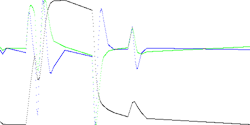
Fig. 3b. TEK00000 model with k = 50.
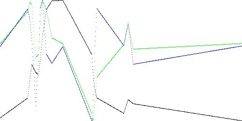
Fig. 3c. TEK00000 model with k = 20.
Note that TSAD4 performs a piecewise linear approximation of a path, not of the original training data. We can get a better fit to the data if we substitute |AC| with tC - tA in equation (1). That is, for points A-B-C we would estimate the length of the line segment AC along the horizontal axis of the above graphs instead of their distance in (x,dx,ddx) space:
error(B) - (tC - tA)d2 (2)where tC - tA is the time between points A and C. Figure 4 below shows this approximation for k = 20. Visually, this would appear to be a better fit than Figure 3c above. However the anomaly detection would be worse, as shown in Table 4 below, when compared with Table 2. In particular, the maximum scores for TEK00002, TEK00003, and TEK00011 would be lower than for the normal trace, TEK00001.
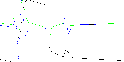
Fig. 4. TEK00000 model using Eq. 2 and k = 20
Table 4.  Hypothetical TEK anomaly scores for k = 20 using Equation (2).

k = 20, Eq. (2)                     Maximum      Total anomaly score
---------------                     --------     -------------------
TEK00001.CSV                        0.027459     1.325680 (normal)
TEK00002.CSV                        0.021483     1.641138
TEK00003.CSV                        0.022381     1.748637
TEK00010.CSV                        0.088797     3.430439
TEK00011.CSV                        0.017170     1.847995
TEK00012.CSV                        0.066348     3.041922
TEK00013.CSV                        0.052866     3.964041
TEK00014.CSV                        0.066641     6.302476
TEK00015.CSV                        0.068445     5.868922
TEK00016.CSV                        0.110843     8.306214
TEK00017.CSV                        0.069369     3.580601
  n = 40000 (2 traces: V37898 V32 T21 R00s.txt and V37898 V32 T21 R01s.txt)
  C = 1 (shunt resistor) or 2 (Hall effect sensor)
  T = 50 (5 ms)
  k = 100 approximation vertices
  m = 3 dimensions
  s = 1 (no subsampling)
In both cases, the normal trace has a lower maximum and total anomaly score than all the abnormal traces. The effect is stronger for the Hall effect sensor, which is less noisy.
                    Table 5.  VT1 anomaly scores

C = 1 (shunt resistor)             Maximum      Total anomaly score
----------------------             --------     -------------------
V37898 V32 T22 R02s.txt            0.000962     1.022259 (normal)
V37898 V32 T70 R03s.txt            0.017078    36.908261 (hot)
V37898 V32 T22 imp045 R01s.txt     0.005793     3.109558 (4.5 mil block)
V37898 V32 T22 imp09 R01s.txt      0.011831     6.320562 (9 mil block)
V37898 V30 T21 R00s.txt            0.003189     7.149981 (30 V)

C = 2 (Hall effect sensor)         Maximum      Total anomaly score
----------------------             --------     -------------------
V37898 V32 T22 R02s.txt            0.000961     0.176745 (normal)
V37898 V32 T70 R03s.txt            0.047534   259.359477 (hot)
V37898 V32 T22 imp045 R01s.txt     0.006391     2.623365 (4.5 mil block)
V37898 V32 T22 imp09 R01s.txt      0.012792     5.731834 (9 mil block)
V37898 V30 T21 R00s.txt            0.004860    12.056552 (30 V)
Execution time was 0.66 seconds to read, filter, compute derivatives for, and store the 40,000 training samples, 0.77 seconds to construct the model, and 4.3 seconds to test 100,000 points (43 uS per test).
  n = 1000000 training samples (first 50 traces)
  C = 1 (shunt resistor)
  T = 50 (5 ms)
  k = 100 vertices
  m = 3 dimensions
  s = 1 (no subsampling)
Execution time was 23.4 seconds to read, filter, store, and compute derivatives of 1,000,000 data points, 30.2 seconds to construct a piecewise linear approximation, and 162.0 seconds to test 3,360,000 data points, producing 203 MB of output data. Testing speed was 48 microseconds per data point, or about 0.5 uS to test a point against one path segment.
The data consists of 20 battery charger simulations with 2 batteries. There are 10 normal traces used for training, and 10 abnormal traces used for testing. For these tests, we monitor battery 1, and consider traces with faults in battery 2 only to be normal. Each trace is about 1000 samples, some with Gaussian noise added. TSAD4 parameters are:
  n = 10134 (10 normal traces, run01 to run10)
  C = 3 (battery 1 voltage) or 4 (battery 1 temperature)
  T = 5 samples
  k = 50 vertices
  m = 3 dimensions
  s = 1 (no subsampling)
Test results are shown below. The normal traces have a lower maximum anomaly score in every case than the corresponding abnormal traces, and lower total anomaly scores with the exception of one trace (run20). This miss was not due to the piecewise approximation, which was verified by setting k = n.
               Table 6.  Battery test anomaly scores.

Battery 1 voltage                      Maximum   Total anomaly score
----------------------                 --------  -------------------
run11_high1_noise0.txt                 1.851946  1577.839295
run12_high2_noise0.txt                 0.883425    18.030273 (normal)
run13_high12_noise0.txt                1.829013  1485.409673
run14_low1_noise0.txt                  0.846310    17.659066
run15_low2_noise0.txt                  0.002036     0.138853 (normal)
run16_high1_noise500.txt               0.672971   156.031874
run17_high2_noise500.txt               0.101400     2.518061 (normal)
run18_high12_noise500.txt              0.596557   141.470954
run19_low1_noise500.txt                0.049823     1.863862
run20_low2_noise500.txt                0.015404     3.472748 (normal)

Battery 1 temperature                  Maximum   Total anomaly score
----------------------                 --------  -------------------
run11_high1_noise0.txt                 1.893265  1663.967716
run12_high2_noise0.txt                 1.004387    19.560402 (normal)
run13_high12_noise0.txt                1.871072  1566.832490
run14_low1_noise0.txt                  0.951641    19.020646
run15_low2_noise0.txt                  0.001681     0.079056 (normal)
run16_high1_noise500.txt               0.886871   210.070683
run17_high2_noise500.txt               0.151140     3.123684 (normal)
run18_high12_noise500.txt              0.801762   190.926153
run19_low1_noise500.txt                0.060495     1.910753
run20_low2_noise500.txt                0.025160     3.773030 (normal)
Execttion times were 0.27 seconds to read and filter the training data, 0.16 seconds to find the piecewise approximation, and 0.44 seconds to test 10,173 points.
In prior work we introduced path modeling for anomaly detection. A path model consists of the points traced by a time series and its m-1 filtered derivatives in m-dimensional space. A test point is anomalous if it is far from the modeled path.
A disadvantage of path modeling is that O(n) time is required to compare a test point to n training points. In this work we reduce the test time to O(k), k << n, to compare to a piecewise approximation of k line segments. The approximation is to remove vertices from the path when they lie near a straight line formed by its neighbors, until only k vertices remain. This method is not optimal (it is greedy) but gives good results in practice. We introduce a fast (O(n log n)) algorithm for performing this approximation using a doubly linked heap.
Path model anomaly detection is sensitive to T (filer time constant), k (number of segments) and m (number of dimensions). For the data tested, m = 3 was found to work best. T defines a "fuzzy window size" over which test data should match a corresponding window somewhere in the training data. The selection of k depends on the complexity of the training data. A training trace with multiple cycles requires higher k. Testing time is proportional to m and k, but does not depend on T.
Piecewise path modeling also solves a second problem, that of providing a concise description of the model for manual editing. A path model can be described in a k by m table of coordinates and can be viewed graphically as an approximation of the original training data. However it should be noted that the best visual fit to the training data is not necessarily the best path model.
[1] S. Salvador, P. Chan, J. Brodie, Learning States and Rules for Time Series Anomaly Detection, Florida Tech TR-CS-2003-05, 2003.